
Introduction
Welcome to the technical documentation for SHIFT (SHeffield Ice Flow Tracker). SHIFT is the processing pipeline we use to derive velocity fields from Sentinel-1 Synthetic Aperture Radar (SAR) image pairs.
4.1. Overview of approach
The velocity fields are derived using intensity tracking algorithms applied to consecutive Sentinel-1 image pairs. Our processing pipeline is fully automated and involves:
- Metadata curation and data download: At least daily, our system collates information about all Sentinel-1 images that have been acquired over Greenland and Antarctica and identifies all potential image pairs. For each available image pair that hasn't yet been processed, it downloads the images, orbital positioning information and digitial elevation models required to complete the processing. All data download and curation is completed 'on-the-fly' to minimise storage requirements.
- Pre-processing: We use the open-source Generic Mapping Tools for Synthetic Aperture Radar (GMTSAR) imagery software to prepare the raw radar images for feature tracking and generate the information required to convert the images from radar to map coordinates. This process ingests the raw radar images, orbital data and elevation data.
- Feature/intensity/speckle tracking: 2D fields of ice velocity are estimated and posted at 150x150 m resolution using standard methods.
- Post-processing: Individual velocity fields are filtered to remove outliers, which are defined using cross-correlation quality metrics and based on the characteristics of the retrieved flow field.
- Mosaic creation: The 'raw' velocity fields derived from Sentinel-1 swaths are geocoded to a common grid then further corrections and outlier removal routines are applied.
4.2. Data Sources
Sentinel-1: The European Space Agency (ESA) Sentinel-1 missions comprise a constellation of two sun-synchronous polar-orbiting satellites, which operate in the same orbital plane with 180 degree phasing difference. They perform C-band Synthetic Aperture Radar (SAR) imaging, enabling day and night acquisitions regardless of weather.
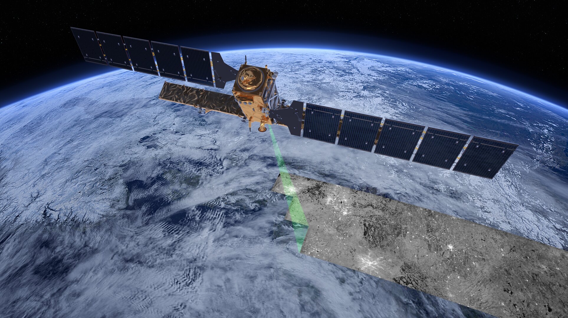
What is a radar image? Radar imaging is an "active" data collection technique where the satellite radar transmits its own pulses of energy and records the amount reflected back from the Earth's surface - surfaces that reflect more energy back appear brighter. Typically, rougher surfaces and surfaces oriented towards the incoming radar waves appear brighter than smooth surfaces or those that are facing away from the sensor. Surface properties also affect how much of the incoming radar signal is returned to the satellite: crucially for glaciers, a smooth wet surface (as might be expected on glaciers during summer), acts as a 'specular reflector', which causes the radar waves to reflect away from the satellite and makes water appear dark in radar imagery. This all differs from optical imagery, which relies on passive light from the sun.
For our processing with SHIFT, we use Sentinel-1 Level-1 Single Look Complex (SLC) images. SLC images represent the 'raw' radar returns from the ground surface, processed into a 2D image, but before those radar returns have been projected onto the ground surface. Since it has not been projected, the raw SLC image is in 'slant range' or 'line-of-sight' geometry, as if you are viewing the surface from the perspective of the satellite antenna without knowing anything about the ground topography. As part of our processing, we also produce ground-projected radar amplitude images (as shown in Fig. 4.2).
Sentinel-1A was launched on 3 April 2014, Sentinel-1B was launched on 25 April 2016, Sentinel-1C was launched on 5 December 2024 and Sentinel-1D was launched on 4 November 2025. Sentinel-1B experienced a failure of the power supply. on 23 December 2021, leaving it unable to deliver images.
Each of these individual satellites orbits the Earth in a consistent pattern. This allows them to image the same location on the ground every 12-days (so-called 'repeat' imagery). Since each pair of satellites orbit the Earth 180 degrees apart but in the same orbital plane, we can combine the images from pairs of Sentinel-1 satellites to acquire repeat images every six days. Since our ice velocity measurements require us to measure the movement of surface features over some time period, this repeat image acquisition time period means that our velocity measurements represent the average ice speed during the time period between image acquisitions (which must be a multiple of six days). The Sentinel-1 SAR instrument can acquire images in four exclusive modes:
- Stripmap: the standard mode.
- Interferometric Wide (IW) swath: where three 'swaths' of data are acquired using the TOPSAR technique.
- Extra Wide swath: where five 'swaths' of data are acquired using the TOPSAR technique, but at lower resolution to the IW mode.
- Wave: where small 'vignettes' of data are acquired at 100 km along-track intervals, alternating between near- and far-range incidence angles.
For our processing with SHIFT, we use images acquired in Interferometric Wide swath mode.
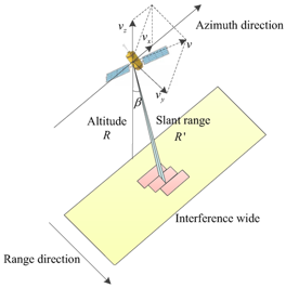
What is Synthetic Aperture Radar (SAR)? Synthetic Aperture Radar (SAR) is a way of acquiring radar images that increases their spatial resolution. The resolution of a radar imaging system depends, among other things, on the length of the antenna - longer antennas provide higher resolutions and therefore more detailed imagery. To achieve high-resolution images (meaning images with pixel dimensions of several metres) from space, a standard radar would require an impractically large antenna (over 4,000 meters long for C-band radar!). SAR solves this by using the motion of the satellite to simulate a much larger antenna. By combining a sequence of signals received as the satellite moves along its flight path, it creates a "synthetic aperture" that produces high-resolution data from a physically small antenna. You can read more about SAR here.
Sentinel-1 Single Look Complex (SLC) data are provided in various polarisation, but HH (horizontal emit and horizontal receive) is best for ice velocity estimation.
4.3. Pre-processing
We use GMTSAR to convert Sentinel-1 SLC IW image pairs to co-registered, geocoded amplitude images suitable for feature tracking. In the following, the first and second image in the image pair is referred to as image1 and image2, respectively.
- Geometric alignment, deramping and burst stitching: We use information about the satellite position and the ground surface to align image2 with image1. Deramping removes the phase ramp inherent in TOPS (Terrain Observation with Progressive Scans) data, resulting from the steering of the antenna beam during acquisition, to ensure phase continuity. Two levels of orbital information are available: 'Precise' and 'Restituted' orbits. Precise orbits are accurate to 5 cm but are only available 21 days after image acquisition. Restituted orbits are accurate to 10 cm and are available within 3 hours of image acquisition. Wherever possible, we use the precise orbits. In practice, the choice of orbit information has no discernable impact on the retrieved velocity field. We then stitch bursts together to form three sub-swaths per image pair. We use a fixed map of the ice surface provided by Digitial Elevation Models (DEMs). For the Antarctic Peninsula, we use the 100 m REMA DEM mosaic, whilst for Greenland we use the 90 m Greenland Ice Mapping Project DEM.
- Geocoding of amplitude: Once the complex images are prepared, we extract the amplitude component. Then we calculate a transformation function between radar coordinates and geographic coordinates, accounting for elevation and time. We retain the image in radar coordinates until after the feature tracking is complete.
Prior to feature tracking, we apply a Contrast-Limited Adaptive Histogram Equalization filter to the pre-prepared amplitude images to maximize the visibility of surface features.
4.4. Measurement Algorithms
Our core processing pipeline is adapted from, (PIVSuite) which was inspired by (PIVLab). We use fairly standard "feature tracking" approaches to measure the displacement of ice surface features between two co-registered SAR images.
4.4.1. Interrogation Areas (IAs)
Feature tracking does not track every individual ground feature. Instead, the image1 and image2 are divided into small sub-images called Interrogation Areas (IAs).
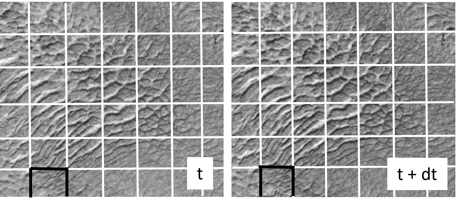
The size and distribution of these IAs are critical tunable parameters:
- IA Size: The window size (e.g., 64x64 or 128x128 pixels). Larger IAs contain more distinct features, typically providing a stronger correlation signal, but they effectively "average" the velocity over a larger area. Smaller IAs measure displacement over smaller areas, but are more susceptible to noise or "loss of correlation". Since Sentinel-1 images have different resolutions in the range (line-of-sight) and azimuth (along-flight or along-track) directions (nominally 2.3 x 14.1 m), we use different IA lengths in each direction. In general, it is recommended that the dimensions of the IA should be at least four times the maximum expected displacement.
- Step Size (Overlap): To produce a smooth velocity map, IAs can (and should!) overlap. For example, if the IA size is 128 pixels, we might step the grid by only 32 pixels. This produces a dense grid of velocity vectors. Typically, the step will be 25% or less of the IA size; we use a step of 12.5% of the IA dimensions. Note: Higher overlap increases the computational cost linearly with the number of generated IAs.
4.4.2. Frequency Domain Cross-Correlation
Calculating the correlation by physically sliding the IA over the search area (Spatial Cross-Correlation) is computationally expensive, with a complexity of O(N2). Instead, we perform Circular Cross-Correlation in the frequency domain using the Fast Fourier Transform (FFT).
According to the Convolution Theorem, the cross-correlation of two functions is equivalent to the multiplication of their Fourier Transforms. For each IA pair, we calculate the 2D cross-correlation surface (Rcorr) as:
Where F denotes the Fourier Transform and * denotes the complex conjugate. Before transformation, windowing functions (e.g., Hanning, Gaussian) are applied to the IAs to reduce spectral leakage caused by edge discontinuities.
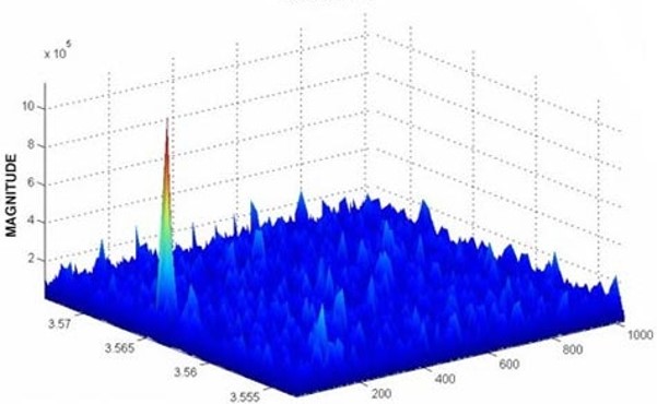
The result is a 2D surface of the magnitude of the correlation strength between image1 and image2, depending on the displacement applied to image1. The correlation at any (x,y) location within the 2D surface can be between -1 and 1. The largest value - the signal - is where the correlation between the two IAs is greatest, so the distance between the centre of the IA to the centre of the cross-correlation peak should correspond to the average displacement between image1 and image2. The mean of the absolute values of the remainder of the 2D cross-correlation surface is referred to as the noise. Therefore, the ratio of the cross-correlation peak magnitude and the noise is called the signal-to-noise ratio or SNR. Low SNR values indicate low confidence (e.g., in areas of featureless snow), allowing us to filter out bad data during post-processing.
Note: In reality, there may be spatial variations of ice speed within the IA. These are not resolved.
4.4.3. Sub-Pixel Peak Finding
Integer-level precision is insufficient for measuring ice motion. To illustrate, imagine the true displacement over a 6-day period is 1.25 pixels in the range direction, where each pixel is 2.3 m in that direction (so 2.875 m of displacement). That is equivalent to a speed of 175 m/yr. Now imagine we only measured the location of the cross-correlation peak to the nearest pixel. That would give 1 pixel or 2.3 m of displacement, which is 140 m/yr and a 20% error! The error is greater in the azimuth direction because the pixel sizes are larger, but lower over 12-day periods because the error per day is less.
To achieve sub-pixel accuracy, we implement the matrix-multiply DFT approach described by Guizar-Sicairos et al. (2008).
Rather than zero-padding the entire FFT (which is memory intensive), this algorithm computes the discrete Fourier transform (DFT) only in a small neighborhood around the initial integer peak. This effectively "zooms in" on the peak in the frequency domain, allowing us to locate the maximum with precision of 1/50th of a pixel, with minimal computational overhead.
4.4.4. Advanced Refinements
To tackle areas of complex ice flow or areas with particularly low signal-to-noise ratio, our workflow supports advanced iterative methods:
- Multi-pass Processing: We perform an initial coarse tracking pass. The resulting velocity estimates are used to pre-shift the IAs for a second, finer pass. This compensates for large displacements and improves correlation.
- Iterative Shifting & Noise Injection: To prevent "pixel locking" (where velocities bias toward integer values), we can iteratively shift the IA position slightly or inject low-level noise, averaging the results to smooth out quantization errors.
4.5. Post-processing
Raw velocity fields derived from feature tracking inevitably contain noise and artifacts caused by ionospheric streaks, featureless surfaces (like fresh snow), or decorrelation. Our post-processing pipeline cleans this data in three distinct stages.
4.5.1. Stage 1: Segmentation Filtering (Radar Geometry)
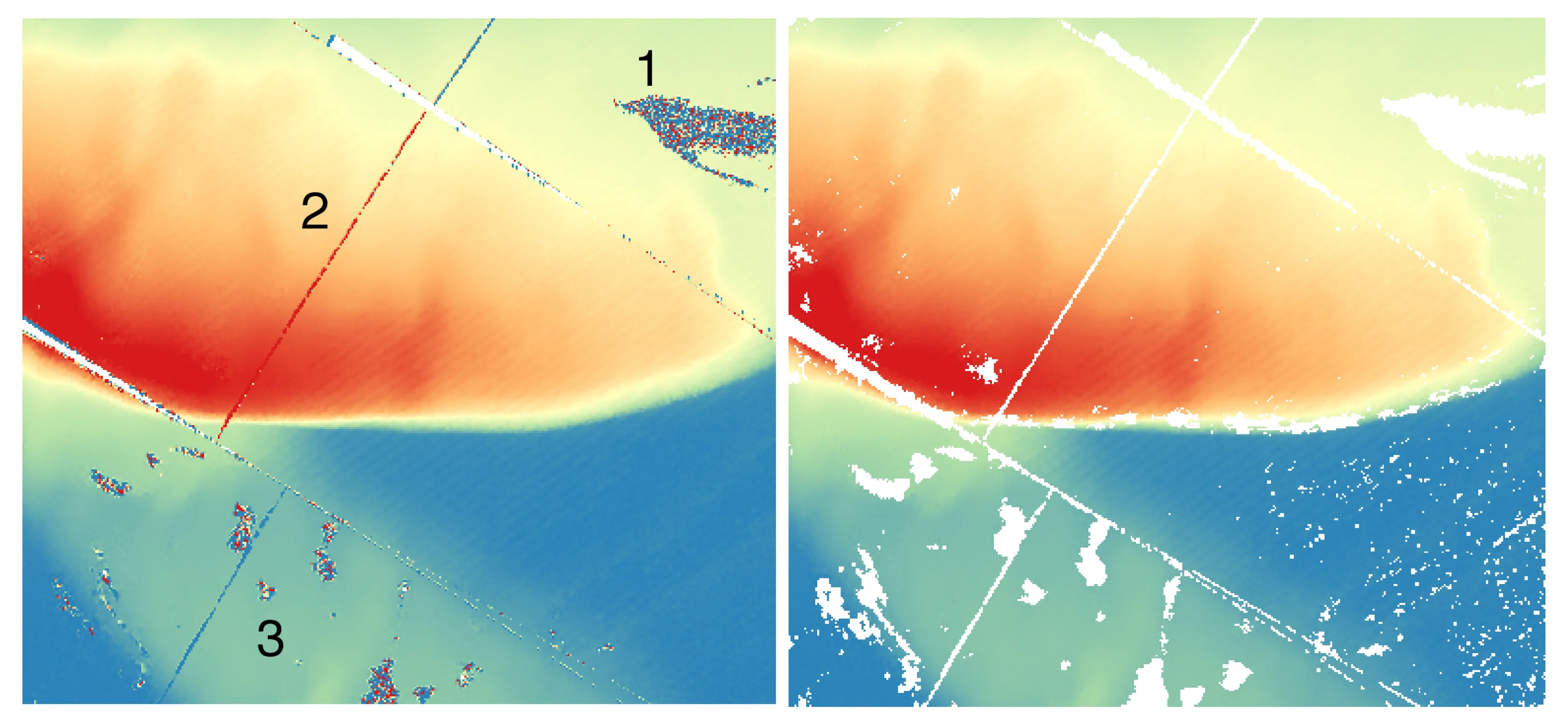
Before geocoding, we apply an image segmentation filter based on the premise that real ice flow is usually smoothly varying. While velocity can change, "islands" of flow surrounded by areas of extremely high strain (rapid changes in speed) are typically erroneous.
We utilize a Region Growing algorithm to identify regions of unphysically rapid velocity change surrounding relatively small groups of pixels. This allows us to identify and remove small groups of pixels separated from the main velocity field by a sharp discontinuity (a 'cliff' in velocity values). The effect of this is to retain a smoothly varying velocity field comprised mostly of large contiguous pixel groups whilst retaining realitic areas of steep speed gradients (such as ice falls and shear margins). This approach adapts the segmentation method described by Luttig et al. (2017).
4.5.2. Stage 2: Ionospheric Destriping
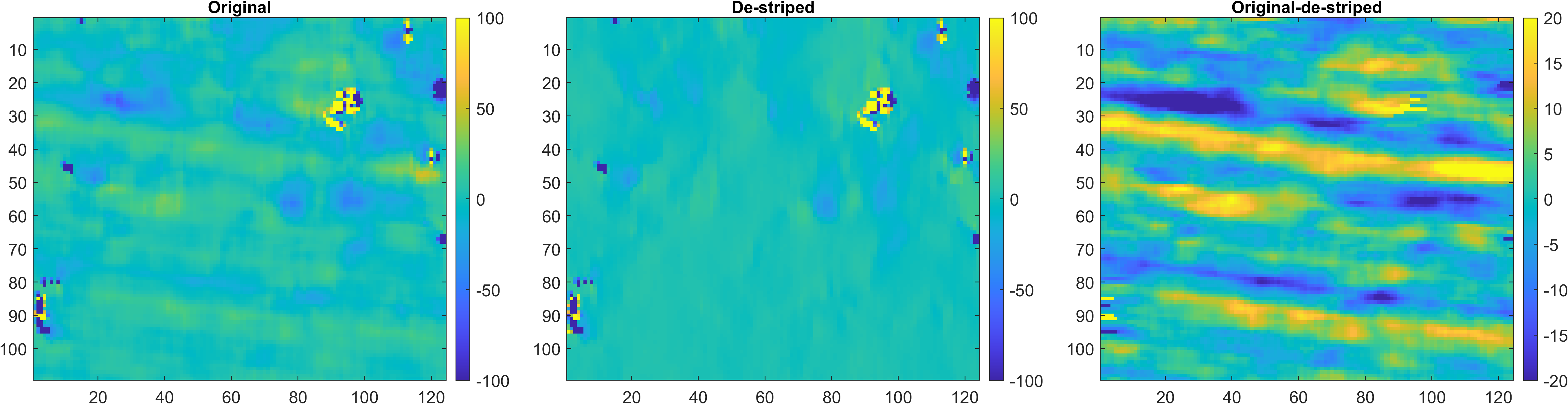
Velocity fields derived from Synthetic Aperture Radar data often suffer from 'striping' artifacts caused by ionospheric irregularities interfering with the radar signal.
We conditonally apply a general destriping algorithm described by Rottmayer et al. (2025).
4.5.3. Stage 3: Map Projection & Outlier Removal
Once the data are cleaned in radar coordinates, they are projected onto the ground surface map geometry. This converts displacements from "pixels" into "meters" and corrects for topographic distortion.
We then run a final suite of physical and statistical filters, always attempting to remove outliers whilst minimising loss of 'good' data:
- Signal-to-Noise Ratio (SNR): We reject any vectors where the cross-correlation peak strength is low relative to the noise floor. We utilize a threshold of SNR > 5.8, (i.e. velocity estimates with an SNR of less than 5.8 are removed). This threshold was established as a robust cutoff for feature tracking by de Lange et al. (2007).
- Flow Direction Filter: Vectors indicating physically impossible flow direction changes (e.g., a sudden reversal in direction) are removed.
- Grubbs Outlier Detection: A statistical test that identifies and removes values that deviate significantly from the local mean (spatial outliers).
- Spatial Isolation: Any remaining vectors that are completely isolated (lacking neighbors) are removed as probable noise.
Finally, small gaps in the remaining velocity field are filled by solving the Dirichlet boundary value problem for the discrete Laplacian over the region of the gap. In the resulting filled area, each filled pixel equals the average of its four immediate neighbours. This produces a smooth interpolation that preserved local flow gradients, rather than introducing artificial flat spots.
4.6. Mosaics
The processing steps described so far operate on individual Sentinel-1 image pairs, each comprised of three 'swaths'. A single acquisition date pair (e.g., June 20 to June 26) may consist of multiple image pairs.
While these swaths share the same map projection, they exist on different pixel grids based on the satellite's specific track. To create an analysis-ready product, we must standardize all these swath-based velocity fields onto a common grid. We achieve this by generating date-pair mosaics.
4.6.1. "Raw" Mosaics
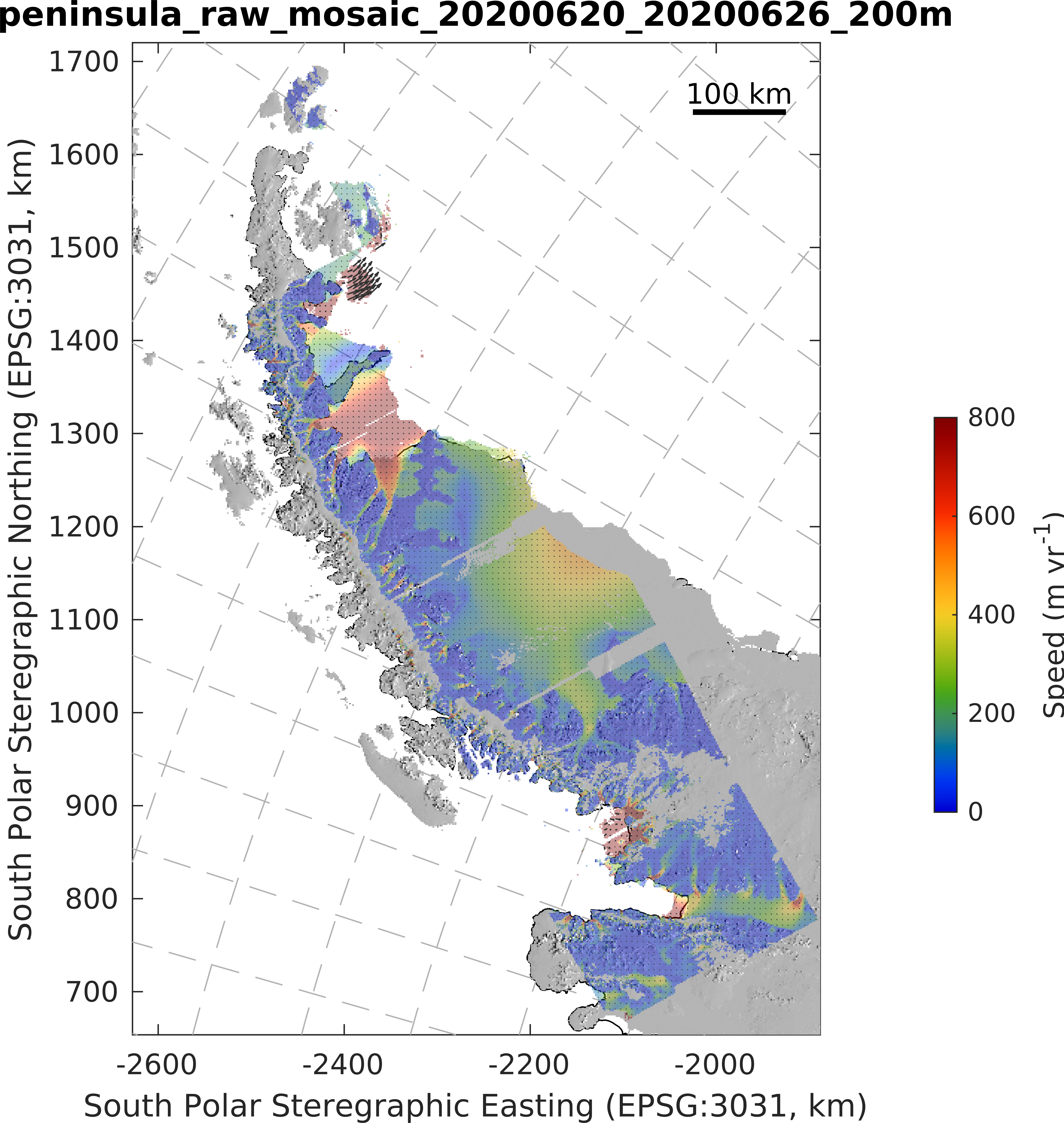
The "Raw" mosaic process aggregates all velocity data derived from any Sentinel-1 pair covering the same time window (e.g., all data measuring displacement between Date A and Date B). It also removes offsets in velocity estimates between overlapping swaths and removed biases detected in bedrock areas (where zero motion is expected, but not always measured).
Step 1: Common Grid Projection
We define a master 'Common Grid' that covers the entire study area (e.g., the full Antarctic Peninsula or West Greenland). Using GDAL (Geospatial Data Abstraction Library) tools, every individual swath is geocoded onto this fixed grid. This ensures that a pixel at index (x, y) in one mosaic corresponds exactly to the same geographic location in every other mosaic in the time series. This grid was defined based on the maximum extent of all available Sentinel-1 image pairs in the two study areas.
Step 2: Merging and Overlap Correction
Sentinel-1 swaths acquired as part of the same image pair overlap. During the mosaicking process, we correct for detected offsets between overlapping swaths if the velocity field is of sufficient quality and the calculated offset is succiently clear. All applied swath offsets are 'tied' to swaths that overlap with bedrock areas.
- Swath Stitching: Adjacent swaths (from the same image pair) are stitched together.
- Image Pair Merging: If multiple image pairs were acquired on the same day, they are merged. These may or may not overlap.
Step 3: Error and bias correction
Errors in the resulting velocity fields may stem from errors in the calculated satellite position, errors caused by ionospheric interference with the radar wave, errors in the DEM used for projection of the radar image and conversion of displacement field to metres, errors in image co-registration, uncertainties associated with calculation of ice motion over 2D IAs, uncertainties in the calculation of the cross-correlation peak location. These errors are hard to quantify on a pixel-by-pixel basis.
To obtain a measure of the error in our velocity estimates we use two metrics. The first is simply the SNR of the cross-correlation field for each IA, which we also produce date-pair mosaics of. The second is the apparent deviation from zero motion across bedrock areas in velocity fields containing bedrock. In west Greenland, large areas of bedrock are available. Less is available on the Antarctic Peninsula. When forming the mosaics, we calculate the median velocity of bedrock areas and apply that as a bias correction to the mosaics and we retain that motion as a measure of the 'global' error in each date-pair mosaic.
Step 4: Spatial Filtering
Once merged and bias-corrected, we apply a Hybrid Median Filter to the mosaic. This filter is specifically chosen because it effectively removes "salt-and-pepper" noise (random, high-frequency outliers) in the data, while preserving sharp edges - crucial for maintaining the distinct boundaries of shear margins in ice streams. We then fill small spatial gaps in each mosaic.
The result of this process is what we term a raw date-pair mosaic: a spatially continuous, calibrated velocity map on a standardized grid. As you can see from the above processing steps, many filters using spatial information have been applied, so it is not truly raw.
4.6.2. Time-Filtered Mosaics
While the "Raw" mosaics provide a spatially continuous view for specific date pairs, we further reduce noise by using time-series information in each spatial cell.
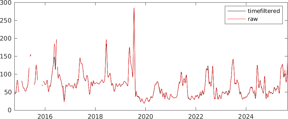
To produce these time-filtered mosaics, we exploit the high temporal frequency of Sentinel-1. By stacking every available mosaic into a 3D cube (Dimensions: x, y, time), we can analyze the history of every single pixel. This allows us to differentiate between transient noise (random spikes) and real geophysical signals (such as seasonal speedups or glacial surges).
We apply three distinct filters in the temporal domain:
Step 1. Velocity Magnitude Outlier Detection
This filter examines the speed at a single pixel location over the entire record. It identifies and removes data points where the velocity deviates statistically from the local temporal trend.
- Method: We utilize MATLAB's
isoutlierfunction. Depending on the specific region dynamics, we apply either a Hampel Filter (moving median) or a standard Median Absolute Deviation (MAD) test. - Why it works: A sudden, single-date spike in velocity of 500% is physically implausible for a glacier. However, the use of a moving window (Hampel) ensures that gradual changes (like a summer speedup or the onset of a surge) are preserved as valid data.
Step 2. Velocity Gradient Filter (Texture Consistency)
Sometimes, an entire scene may be contaminated by noise that produces velocity values within a "plausible" range, but with an unrealistic spatial texture (e.g., "bumpy" or "jagged" flow) that deviates significantly from the historical mean spatial variations in ice flow.
This filter calculates the spatial gradient (numerical derivative) of the velocity field for every time step. If the spatial gradient of the flow on a specific date is significantly higher than the historical median for that location, the data point is flagged as an outlier. This effectively removes areas where spatial gradients in flow have changed unrealistically.
Step 3. Flow Direction Stability
Ice flow direction is generally constrained by topography and is usually expected to change little or only fairly slowly within the contraints of the imaging platform. We calculate the long-term average flow direction for every pixel. We compare the flow direction of each individual date pair against this long-term average. If the flow direction deviates beyond a physical threshold (indicating sudden and/or unsustained change in flow direction), the velocity estimate in that x,y,time location is removed.
SHIVER provides access to our 'raw' mosaics, because in our experience the most suitable filtering step depends on the application and time period studied, so most researchers prefer to work with data closer to the raw observations.
4.7. Automation
Our processing is automated and powered by the University of Sheffield High Performance Cluster Stanage.
Our complete automation workflow is available in the document below. Much of it is specific to the University of Sheffield HPC cluster, so you won't be able to directly adopt our approach, but we have included it below to outline our approach.
We use a SpatioTemporal Asset Catalog (STAC)-like architecture that defines all available image pairs and their processing status. This STAC is updated at least daily with new images as Sentinel-1 acquires them and as new image pairs are processed by our in-house HPC cluster. The beauty of the STAC is that it allows us to query our full catalogue of velocity swaths (or potential but unprocessed swaths) using any combination of spatial and temporal filtering. It also allows us to record useful processing metadata, such as the progress through each processing stage, the number of processing attempts, and the computing resources (time, RAM, #cores) required to complete each processing stage, which allows us to optimise our resource requests and maximise the 'churn' of image pairs that we can process.
Plus, each day we get a nice new .pdf summarising our processing progress and visualising the latest swaths that have been completed.
4.8. References
Sandwell, D., Mellors, R., Tong, X., Wei, M. and Wessel, P., 2011. GMTSAR: An InSAR processing system based on generic mapping tools.
De Zan, F. and Guarnieri, A.M., 2006. TOPSAR: Terrain observation by progressive scans. IEEE Transactions on Geoscience and Remote Sensing, 44(9), pp.2352-2360.
Jiri Vejrazka (2026). PIVsuite (https://uk.mathworks.com/matlabcentral/fileexchange/45028-pivsuite), MATLAB Central File Exchange. Retrieved April 21, 2026.
Thielicke, W. and Sonntag, R., 2021. Particle Image Velocimetry for MATLAB: Accuracy and enhanced algorithms in PIVlab. Journal of Open Research Software, 9(1).
Guizar-Sicairos, M., Thurman, S.T. and Fienup, J.R., 2008. Efficient subpixel image registration algorithms. Optics letters, 33(2), pp.156-158.
Lüttig, C., Neckel, N. and Humbert, A., 2017. A combined approach for filtering ice surface velocity fields derived from remote sensing methods. Remote Sensing, 9(10), p.1062.
Rottmayer, N., Redenbach, C. and Fahrbach, F.O., 2025. A universal and effective variational method for destriping: application to light-sheet microscopy, FIB-SEM, and remote sensing images. Optics Express, 33(3), pp.5800-5809.
de Lange, R., Luckman, A. and Murray, T., 2007. Improvement of satellite radar feature tracking for ice velocity derivation by spatial frequency filtering. IEEE transactions on geoscience and remote sensing, 45(7), pp.2309-2318.